
Notice
Recent Posts
Recent Comments
Link
| 일 | 월 | 화 | 수 | 목 | 금 | 토 |
|---|---|---|---|---|---|---|
| 1 | 2 | 3 | 4 | 5 | 6 | 7 |
| 8 | 9 | 10 | 11 | 12 | 13 | 14 |
| 15 | 16 | 17 | 18 | 19 | 20 | 21 |
| 22 | 23 | 24 | 25 | 26 | 27 | 28 |
| 29 | 30 |
Tags
- 파이썬
- 월간결산
- Ga
- 텐서플로
- 시각화
- Python
- 파이썬 시각화
- Visualization
- 리눅스
- SQL
- 블로그
- 서평단
- Pandas
- 딥러닝
- 매틀랩
- tensorflow
- MySQL
- Tistory
- 한빛미디어서평단
- Linux
- Google Analytics
- 서평
- 티스토리
- 독후감
- Blog
- matplotlib
- python visualization
- MATLAB
- 한빛미디어
- 통계학
Archives
- Today
- Total
pbj0812의 코딩 일기
[TensorFlow] sin 그래프 예측하기 본문
0. 목표
- TensorFlow를 이용하여 sin 그래프 예측하기
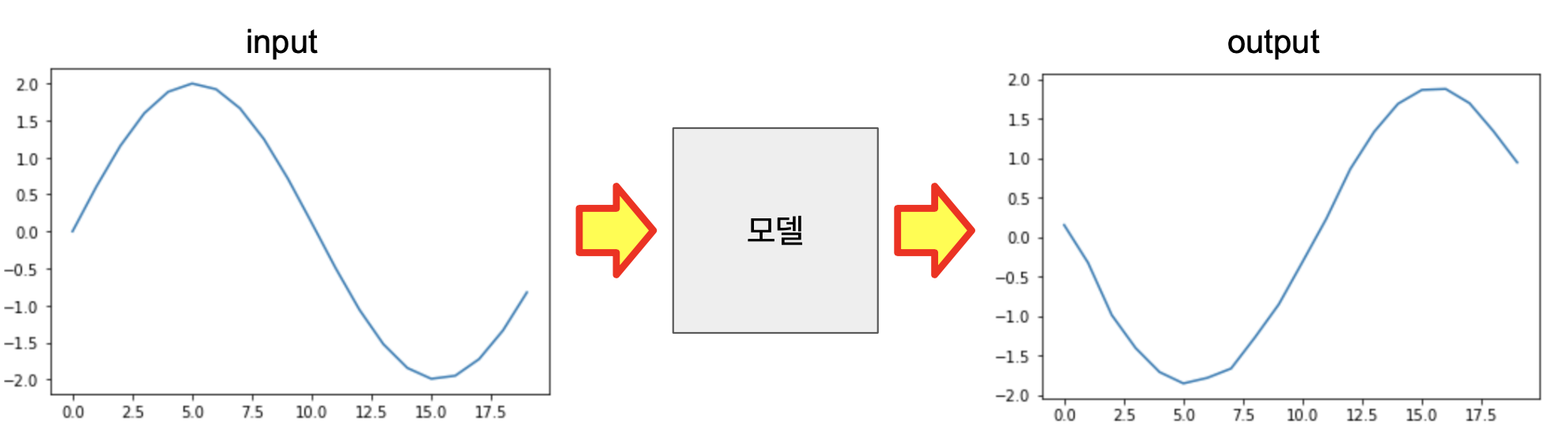
1. FlowChart
- input 값을 넣어주면 그에 따른 sin 그래프를 예측
2. 코드 작성
1) library 호출
import tensorflow as tf
import matplotlib.pyplot as plt
import numpy as np

from tensorflow import keras
from tensorflow.keras import layers
2) 가상 데이터 생성
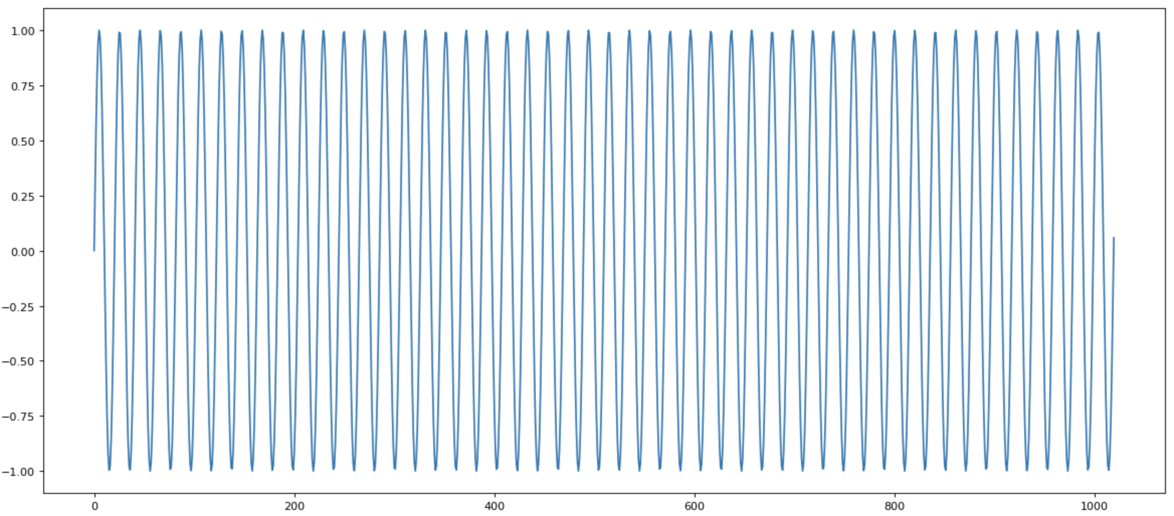
- x : 0 ~ 101*pi 를 1030 등분한 데이터를 삽입
- y : sin(x)
x = np.linspace(0, 101*np.pi, 1030)
y = np.sin(x)
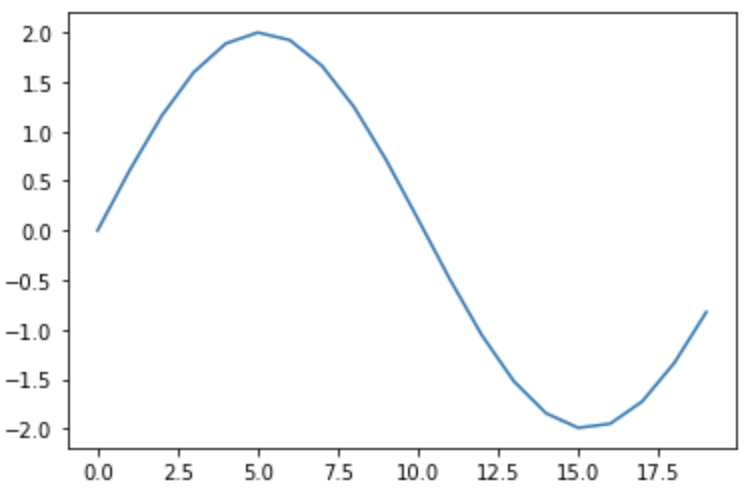
fig=plt.figure(figsize=(18, 8), dpi= 80, facecolor='w', edgecolor='k')
plt.plot(x, y)- 형태

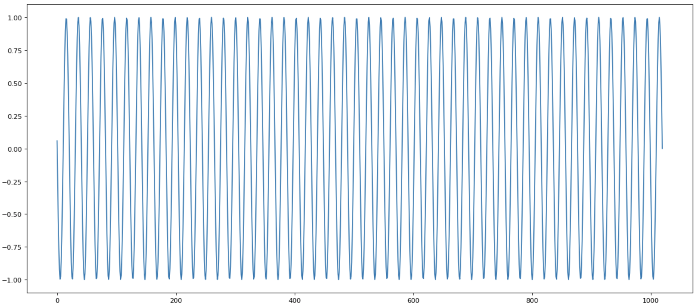
3) 인풋 데이터, 라벨링 데이터 생성
- 인풋은 처음부터 뒤에서 10칸 모자르게, 라벨링은 11번째 데이터부터 끝까지
train_x = y[:1020]
train_y = y[10:]
print(len(train_x))
print(len(train_y))
- train_x
- train_y
4) 학습용 인풋 생성 함수 제작
- 20개씩 쌍으로 생성
- 한칸씩 윈도우가 밀려나면서 저장하는 형태
def MakeInput(x):
  result = []
  for i in range(len(x) - 20):
    result.append(x[i:i+20])
  result = np.reshape(result, (1000, 20, 1))
  return result
5) 인풋 데이터, 라벨링 데이터를 인풋 형태로 변환
- 둘다 (1000, 20, 1)의 형태
train_x2 = MakeInput(train_x)
train_y2 = MakeInput(train_y)
6) 모델 생성
- 인풋에 20개씩 들어가도록 생성
- 아웃풋도 20개
model = tf.keras.models.Sequential([
  tf.keras.layers.Flatten(input_shape=(20, 1)),
  tf.keras.layers.Dense(128, activation='relu'),
  tf.keras.layers.Dense(128, activation='relu'),
  tf.keras.layers.Dense(20, activation='linear')
])
7) 모델 컴파일
optimizer = tf.keras.optimizers.RMSprop(0.001)
model.compile(loss='mse',
                optimizer=optimizer,
                metrics='mse')
8) 생성모델 확인
model.summary()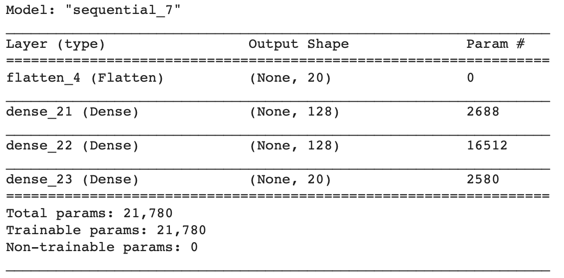
9) 모델 학습
model.fit(train_x2, train_y2, epochs=100)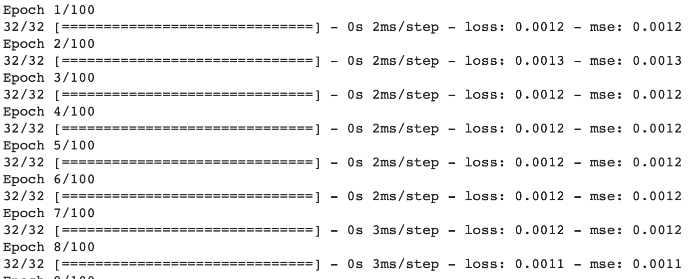
10) 새로운 데이터로 모델 예측
- 위와 같은 방식으로 데이터를 제작하는 대신 값에 2를 곱하여 다른 데이터로 변형
- real_result에 비교할 값을 미리 저장
x2 = np.linspace(0, 101*np.pi, 1030)
y2 = np.sin(x) * 2
print(len(y2))
test_x = y2[:1020]
real_result = y2[10:30]
test_x2 = MakeInput(test_x)
test_x3 = test_x2[0]
test_x4 = np.reshape(test_x3, (1, 20, 1))
- 인풋 데이터 확인
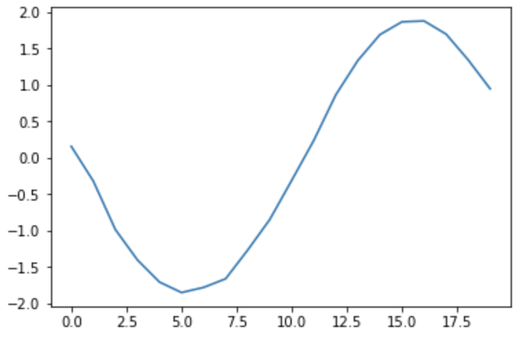
11) 예측
result = model.predict(test_x4)
plt.plot(result[0])
- 결과 확인
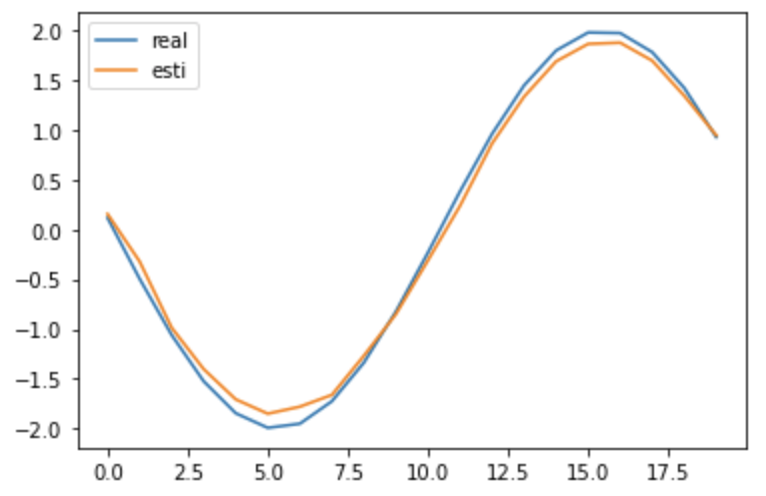
12) 실제값과 비교
plt.plot(real_result, label = 'real')
plt.plot(result[0], label = 'esti')
plt.legend()
- 그림
3. 한계
- 변형하는 형태 sin(x) + b 로 결과 예측시 값이 제대로 나오지 않음 => 학습 데이터가 절편이 없는 형태이기에 그렇게 학습???
4. 참고
- 다중그래프
'인공지능 & 머신러닝 > TensorFlow' 카테고리의 다른 글
| [Tensorflow] node.js & tensorflow.js 를 통한 이미지 판별기 튜토리얼 (0) | 2021.01.04 |
|---|---|
| [TensorFlow] LSTM을 활용한 긍부정 판별기 (0) | 2020.08.11 |
| [TensorFlow] MNIST 예제를 활용한 내가 쓴 숫자 맞추기 (0) | 2020.07.13 |
| [TensorFlow] Colab 세팅하기 (0) | 2020.07.04 |
| [TensorFlow] Sequences, Time Series and Prediction (coursera) (0) | 2020.04.03 |
'인공지능 & 머신러닝/TensorFlow' Related Articles
more


Comments